Overview
Power Electronic Converter Blocks (pecblocks) use the output of detailed electromagnetic transient (EMT) simulations to produce generalized block diagram models of power electronic systems. The process uses deep learning with customized block architectures. The outputs are reduced-order models that meet specified accuracy requirements, while providing important advantages over the original EMT models:
Converter Block models have fewer nodes and can take longer time steps, resulting in shorter simulation times
Converter Block models are continuously differentiable, making them compatible with control design methods
Models will run in both time domain and frequency domain. The scope includes not only the power electronic converter, but also the photovoltaic (PV) array, maximum power point tracking (MPPT), phase-lock loop (PLL) control, output filter circuits, battery storage if present, etc. The applications include but may not be limited to solar power inverters, energy storage converters, motor drives, and other power electronics equipment.
Background
For technical background on pecblocks, see IEEE eGRID 2024 preprint (Table I corrections in red) © 2024 IEEE.
For a control systems application, see SysDO 2024 preprint
For technical background on dynoNet, see Forgione, Piga Paper
For technical background on grid-forming inverters, see Rathnayake, et. al.
Installation
To install the Python package:
pip install pecblocks
Quick Start
The package includes two examples. To download and run them:
Download the Source Distribution from PyPi
Unzip the examples directory from that archive to your local computer. There should be two subdirectories therein:
examples/training contains the files to train an example HWPV model
examples/sdomain contains the files to run a time-domain simulation of a trained HWPV model.
Training a Model
From the examples/training directory:
download
train ucf3
The first command will download a 90-MB sample data file. The second command trains a model, which will take several minutes. Introductory information appears, then a progress log:
Epoch 1420 of 2000 | TrLoss 0.002372 | VldLoss 0.002475 | SensLoss 0.000000 | RMSE 0.0097 | Sigma 0.0000
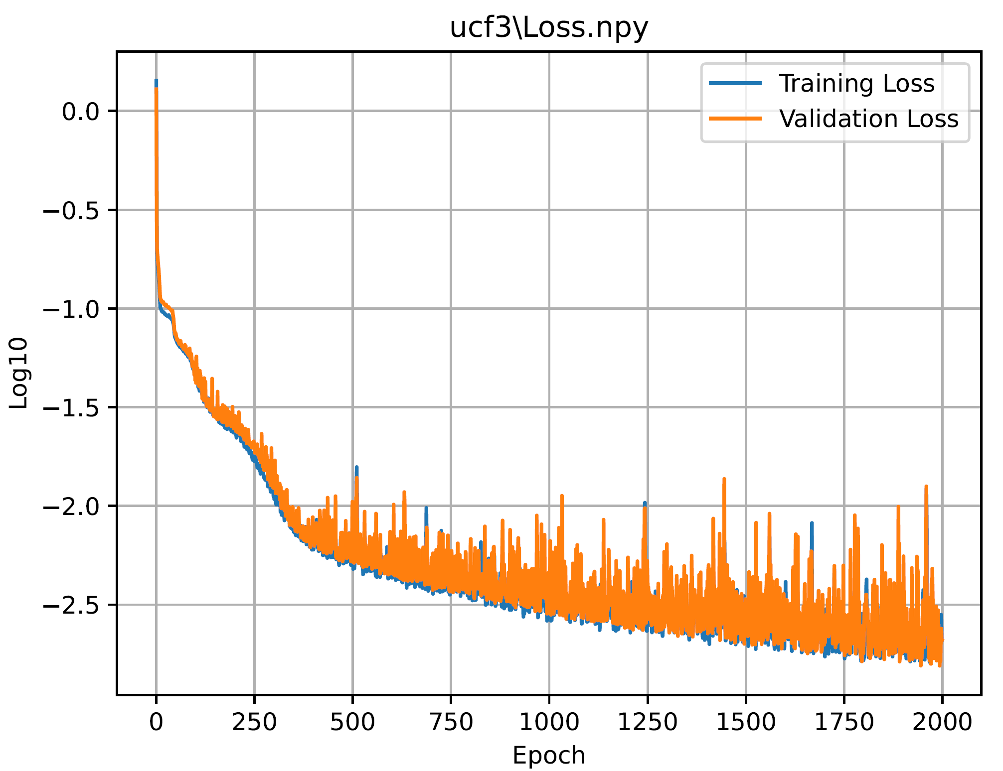
The training loss (TrLoss) and validation loss (VldLoss) should decrease over time, and approach the same order of magnitude. The RMSE represents a root mean square error over all output channels. The goal is for RMSE < 0.05 Even when the logged values are below 0.05, some output channels may exceed 0.05, so the log is just a general indicator of the fitting error. SensLoss and Sigma are zero in this example because no attempt is made to optimize the dq-axis sensitivities between AC voltages and currents.
When training completes, the examples/training/ucf3/summary.txt file should look like this:
Dataset Summary: (Mean=Offset, Range=Scale)
Column       Min       Max      Mean     Range
G         -0.000   999.995   811.581   999.995
Ud         0.800     1.200     1.011     0.400
Uq        -0.499     0.501    -0.006     1.000
Vd         0.000   337.082   219.318   337.082
Vq      -150.297   139.415    -6.328   289.712
GVrms     -0.000 414899.656 253630.828 414899.656
Ctrl       0.000     1.000     0.748     1.000
Vdc        0.000   628.176   461.755   628.176
Idc        0.000     4.834     1.992     4.834
Id         0.000     5.783     2.681     5.783
Iq        -2.635     2.342    -0.080     4.977
COL_Y ['Vdc', 'Idc', 'Id', 'Iq']
Train time: 1539.16, Recent loss: 0.002186, RMS Errors: 0.0030 0.0116 0.0111 0.0047
All four output channels have RMSE < 0.05.
The loss plot in examples/training/ucf3/ucf3_train_loss.pdf should look like this:
Then export the trained model for s-domain simulations:
export ucf3
Some important results of this export appear in examples/training/ucf3/metrics.txt. In the top section:
Read Model from: ./ucf3/
Export Model to: ./ucf3/ucf3_fhf.json
idx_in [0, 1, 2, 3, 4, 5, 6]
idx_out [7, 8, 9, 10]
make_mimo_block iir
H1s[0][0]  Real Poles: [-114.2569614   -56.88678796] Freqs [Hz]: []
H1s[0][1]  Real Poles: [-132.60159228  -58.71635642] Freqs [Hz]: []
H1s[0][2]  Real Poles: [-98.54142517 -98.54142517] Freqs [Hz]: [9.63376790827413]
H1s[0][3]  Real Poles: [-95.95237076 -95.95237076] Freqs [Hz]: [4.705452200660855]
H1s[1][0]  Real Poles: [-135.80799026  -81.8345316 ] Freqs [Hz]: []
H1s[1][1]  Real Poles: [-99.05355517 -99.05355517] Freqs [Hz]: [4.234559773533419]
H1s[1][2]  Real Poles: [-93.8685894 -93.8685894] Freqs [Hz]: [2.7041085997372196]
H1s[1][3]  Real Poles: [-98.32965601 -98.32965601] Freqs [Hz]: [8.50833798367145]
H1s[2][0]  Real Poles: [-118.25321707  -74.03952537] Freqs [Hz]: []
H1s[2][1]  Real Poles: [-143.31944483  -26.50642794] Freqs [Hz]: []
H1s[2][2]  Real Poles: [-92.25928336 -92.25928336] Freqs [Hz]: [7.307075566267579]
H1s[2][3]  Real Poles: [-126.34298102  -28.01220818] Freqs [Hz]: []
H1s[3][0]  Real Poles: [-127.22251461  -62.11887925] Freqs [Hz]: []
H1s[3][1]  Real Poles: [-102.89434604 -102.89434604] Freqs [Hz]: [3.9716432768384853]
H1s[3][2]  Real Poles: [-104.9091462 -104.9091462] Freqs [Hz]: [4.3754426482151345]
H1s[3][3]  Real Poles: [-126.92004256  -64.34811764] Freqs [Hz]: []
All of the H1(s) poles have negative real parts, so they are stable. Some of these poles are complex conjugate pairs, others are real and distinct pairs. Before using H1(s) in simulation, check that all of its poles are stable.
In the bottom section of examples/training/ucf3/metrics.txt:
1498,0.0031,0.0103,0.0086,0.0139
1499,0.0031,0.0099,0.0087,0.0126
Highest RMSE Cases
Vdc  Max RMSE=  0.0057 at Case 1435; 0 > 0.05
Idc  Max RMSE=  0.0337 at Case 34; 0 > 0.05
Id   Max RMSE=  0.0344 at Case 533; 0 > 0.05
Iq   Max RMSE=  0.0202 at Case 515; 0 > 0.05
Total Error Summary
Vdc  RMSE=  0.0030
Idc  RMSE=  0.0116
Id   RMSE=  0.0111
Iq   RMSE=  0.0047
We can see that none of the 1500 cases have RMSE > 0.05. Case 533 has the highest RMSE value for the output Id. For a Norton model, Id is probably the most important output channel. In the middle of the metrics.txt file, we can find some individual case results for the RMSE of each output channel:
533,0.0030,0.0318,0.0344,0.0106
We can plot the fitting result for this worst case as follows:
python pv3_test.py ucf3_config.json 533
The result looks like:

RMSE values in the plot caption match those in metrics.txt, but the initial values are not exactly zero. The initialization can be improved for simulation, but the RMSE values then may not exactly match the values in metrics.txt. For more information, check the usage documentation from:
python pv3_test.py
Simulating a Model
From the example/sdomain directory:
go.bat or ./go.sh
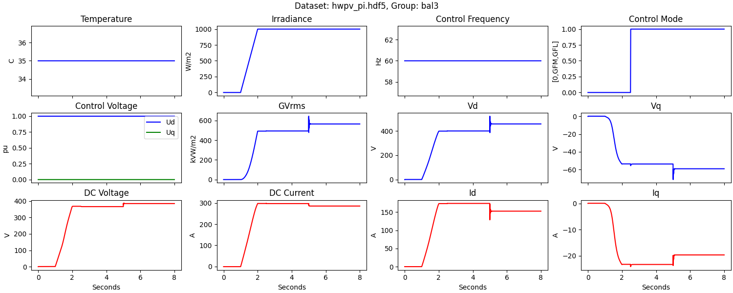
This runs a continous-time simulation of a trained HWPV model for a 100 kW, 480 V inverter. The grid resistance, Rg, begins at 2.3 ohms. The solar irradiance, G, ramps up between 1 and 2 seconds, the control mode changes to GFM at 2.5 seconds, and then Rg changes from 2.3 to 3.0 ohms at 5 seconds. The result looks like:
For more information:
The model in bal3_fhf.json was pre-trained from over 23000 EMT simulations
The Python file hwpv_pi.py illustrates how to test an HWPV model, by application of control inputs, and simulating the effect of external grid resistance, Rg.
The Python file hwpv_evaluator.py implements discrete-time simulation or Euler integration of the model.
Initialization of the Backward Euler method is still under development.
When Rg changes suddenly, as in this example, the time step size is limited to maintain numerical stability. To alleviate this limit, a variable time step for the Euler method is under development.